An Introduction to Topological Data Analysis: Fundamental and Practical Aspects for Data Scientists
Frédéric Chazal, Bertrand Michel
Frontiers in Artificial Intelligence · 2021 · Review · CC BY
doi:10.3389/frai.2021.667963 (opens in a new tab)
We email you when a new notice or a question about this paper appears.
Abstract
With the recent explosion in the amount, the variety, and the dimensionality of available data, identifying, extracting, and exploiting their underlying structure has become a problem of fundamental importance for data analysis and statistical learning. Topological data analysis (tda) is a recent and fast-growing field providing a set of new topological and geometric tools to infer relevant features for possibly complex data. It proposes new well-founded mathematical theories and computational tools that can be used independently or in combination with other data analysis and statistical learning techniques. This article is a brief introduction, through a few selected topics, to basic fundamental and practical aspects of tda for nonexperts.
Abstract licence: CC BY
No text here
Its licence does not allow us to show the full text. Read it at PubMed Central:
Read at PubMed Central (opens in a new tab)Figures14
From PubMed Central, U.S. National Library of Medicine. Licence: CC BY.
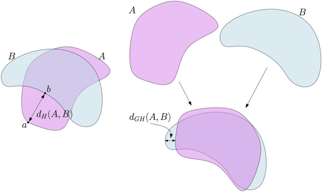
FIGURE 1
Full legend
Left: the Hausdorff distance between two subsets A and B of the plane. In this example, d H (A, B) is the distance between the point a in A which is the farthest from B and its nearest neighbor b on B. Right: the Gromov–Hausdorff distance between A and B. A can be rotated—this is an isometric embedding of A in the plane—to reduce its Hausdorff distance to B. As a consequence, d GH (A, B) ≤ d H (A, B).
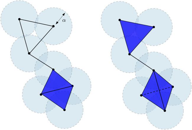
FIGURE 2
Full legend
Čech complex Cechα(X) (left) and the Vietoris–Rips Rips2α(X) (right) of a finite point cloud in the plane R2. The bottom part of Cechα(X) is the union of two adjacent triangles, while the bottom part of Rips2α(X) is the tetrahedron spanned by the four vertices and all its faces. The dimension of the Čech complex is 2. The dimension of the Vietoris–Rips complex is 3. Notice that this latter is thus not embedded in R2.
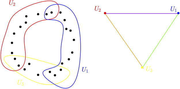
FIGURE 3
Full legend
Point cloud sampled in the plane and a cover of open sets for this point cloud (left). The nerve of this cover is a triangle (right). Edges correspond to a set of the cover whereas a vertex corresponds to a non-empty intersection between two sets of the cover.
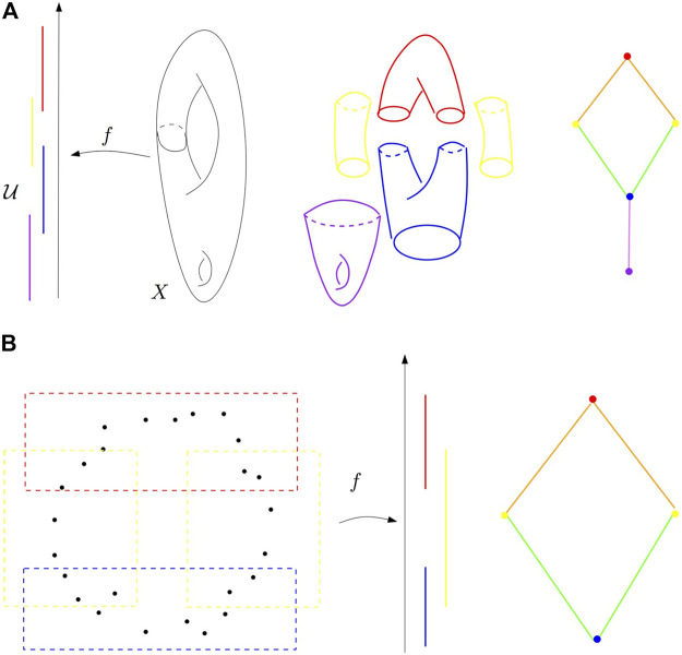
FIGURE 4
Full legend
(A) Refined pull-back cover of the height function on a surface in R3 and its nerve. (B) Mapper algorithm on a point cloud sampled around a circle and the height function. First, the pull-back cover of the height function defined on the point cloud is computed and refined (left). Second, the nerve of the refined pull-back is visualized as a graph (right).
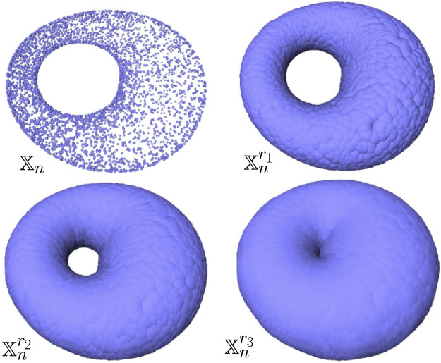
FIGURE 5
Full legend
Example of a point cloud Xn sampled on the surface of a torus in R3 (top left) and its offsets for different values of radii r 1 < r 2 < r 3. For well-chosen values of the radius (e.g., r 1 and r 2), the offsets are clearly homotopy equivalent to a torus.
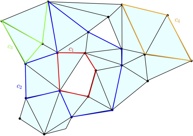
FIGURE 6
Full legend
Some examples of chains, cycles, and boundaries on a two-dimensional complex K: c 1, c 2, and c 4 are one-cycles; c 3 is a one-chain but not a one-cycle; c 4 is the one-boundary, namely, the boundary of the two-chain obtained as the sum of the two triangles surrounded by c 4. The cycles c 1 and c 2 span the same element in H 1(K) as their difference is the two-chain represented by the union of the triangles surrounded by the union of c 1 and c 2.
Show all 14 figures
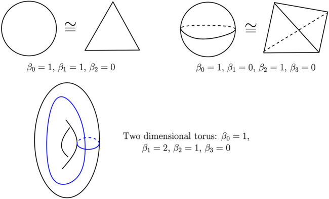
FIGURE 7
Full legend
Betti numbers of the circle (top left), the two-dimensional sphere (top right), and the two-dimensional torus (bottom). The blue curves on the torus represent two independent cycles whose homology class is a basis of its one-dimensional homology group.
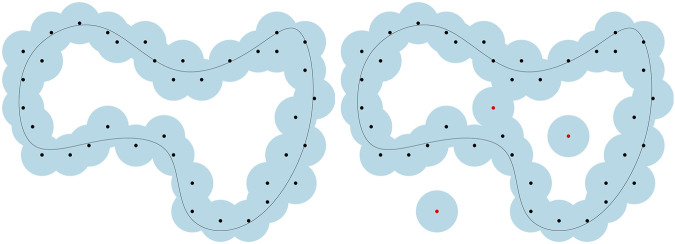
FIGURE 8
Full legend
Effect of outliers on the sublevel sets of distance functions. Adding just a few outliers to a point cloud may dramatically change its distance function and the topology of its offsets.
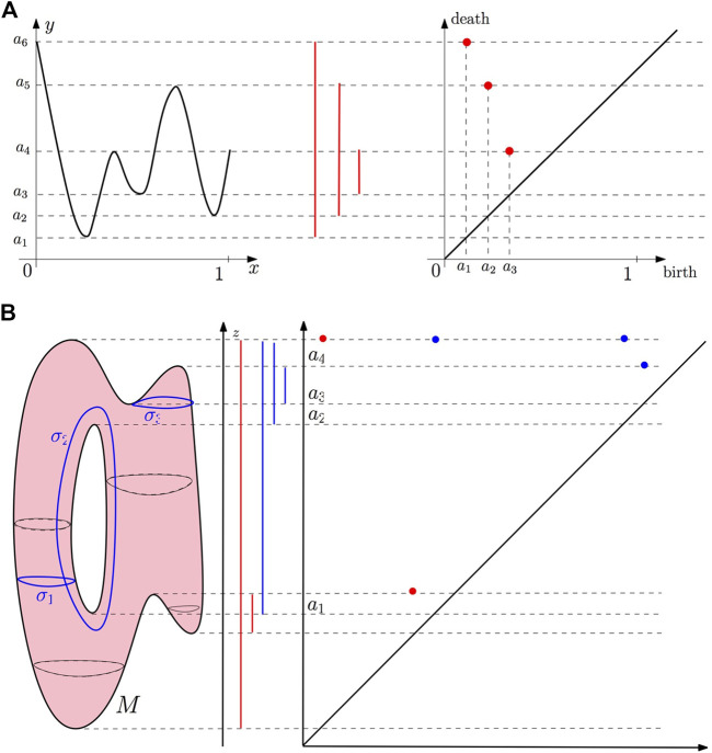
FIGURE 9
Full legend
(A) Example 1: the persistence barcode and the persistence diagram of a function f:[0,1]→R. (B) Example 2: the persistence barcode and the persistence diagram of the height function (projection on the z-axis) defined on a surface in R3.
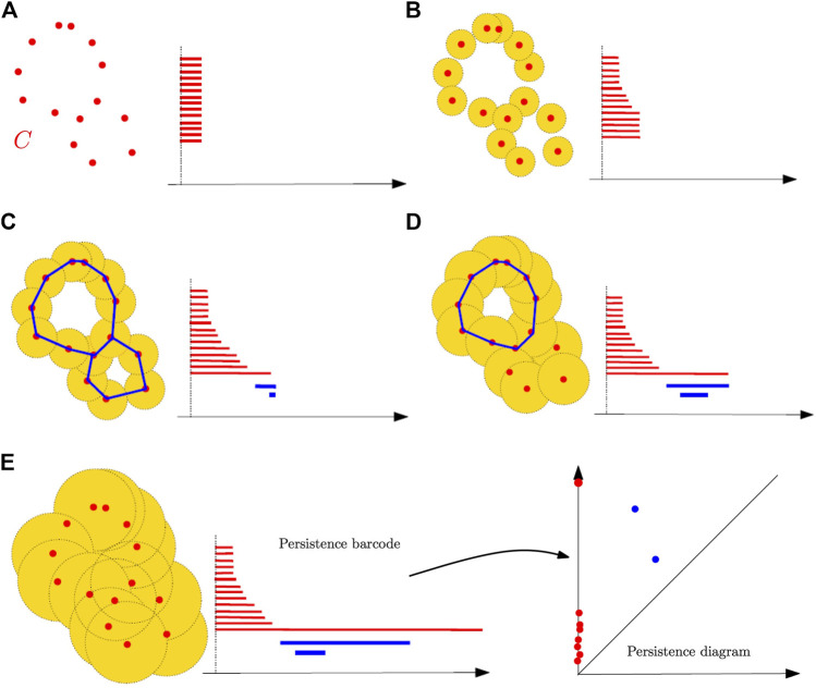
FIGURE 10
Full legend
The sublevel set filtration of the distance function to a point cloud and the construction of its persistence barcode as the radius of balls increases. The blue curves in the unions of balls represent one-cycles associated with the blue bars in the barcodes. The persistence diagram is finally defined from the persistence barcodes. (A) For the radius r = 0, the union of balls is reduced to the initial finite set of points, each of them corresponding to a zero-dimensional feature, that is, a connected component; an interval is created for the birth for each of these features at r = 0. (B) Some of the balls started to overlap, resulting in the death of some connected components that get merged together; the persistence diagram keeps track of these deaths, putting an end point to the corresponding intervals as they disappear. (C) New components have merged, giving rise to a single connected component and, so, all the intervals associated with a zero-dimensional feature have been ended, except the one corresponding to the remaining components; two new one-dimensional features have appeared, resulting in two new intervals (in blue) starting on their birth scale. (D) One of the two one-dimensional cycles has been filled, resulting in its death in the filtration and the end of the corresponding blue interval. (E) All the one-dimensional features have died; only the long (and never dying) red interval remains. As in the previous examples, the final barcode can also be equivalently represented as a persistence diagram where every interval (a, b) is represented by the point of coordinates (a, b) in R2. Intuitively, the longer an interval in the barcode or, equivalently, the farther from the diagonal the corresponding point in the diagram, the more persistent, and thus relevant, the corresponding homological feature across the filtration. Notice also that for a given radius r, the kth Betti number of the corresponding union of balls is equal to the number of persistence intervals corresponding to k-dimensional homological features and containing r. So, the persistence diagram can be seen as a multiscale topological signature encoding the homology of the union of balls for all radii as well as its evolution across the values of r.
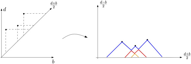
FIGURE 11
Full legend
Example of a persistence landscape (right) associated with a persistence diagram (left). The first landscape is in blue, the second one in red, and the last one in orange. All the other landscapes are zero.
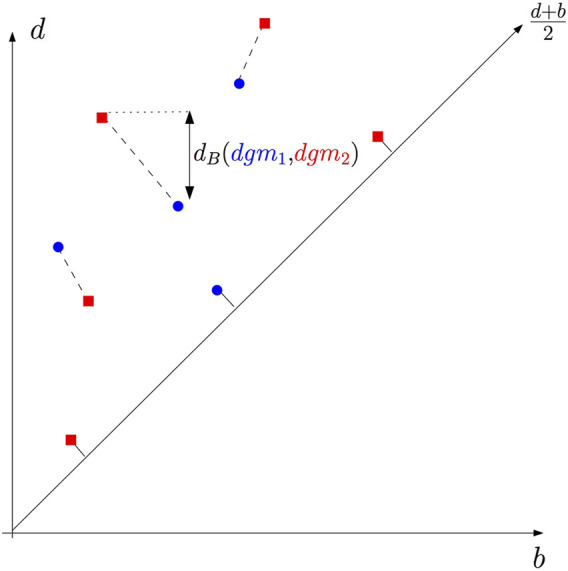
FIGURE 12
Full legend
Perfect matching and the bottleneck distance between a blue and a red diagram. Notice that some points of both diagrams are matched to points of the diagonal.
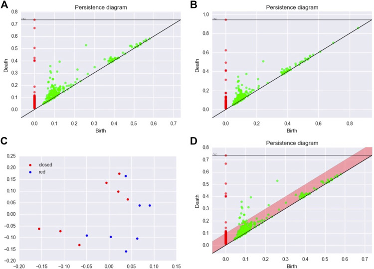
FIGURE 13
Full legend
(A,B) Two persistence diagrams for two configurations of MBP. (C) MDS configuration for the matrix of bottleneck distances. (D) Persistence diagram and confidence region for the persistence diagram of an MBP.
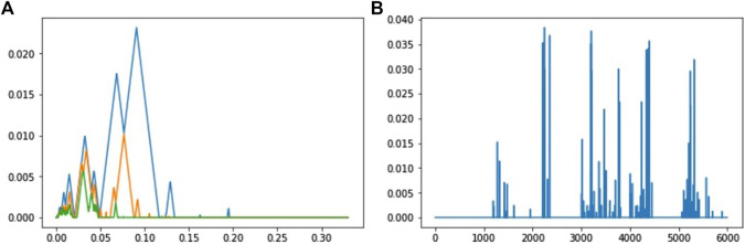
FIGURE 14
Full legend
(A) First three landscapes for zero-homology of the alpha shape filtration defined for a time series of acceleration of Walker A. (B) Variable importances of the landscape coefficients for the classification of walkers. The first 3,000 coefficients correspond to the three landscapes of dimension 0 and the last 3,000 coefficients to the three landscapes of dimension 1. There are 1,000 coefficients per landscape. Note that the first landscape of dimension 0 is always the same using the Rips complex (a trivial landscape), and consequently, the corresponding coefficients have a zero-importance value.
References138
- 1.
Aamari E. Kim J. Chazal F. Michel B. Rinaldo A. Wasserman L. (2019 ). Estimating the Reach of a Manifold. Electron. J. Stat. 13 (1), 1359–1399.
Not in our library10.1214/19-ejs1551 (opens in a new tab)
- 2.
Adams H. Emerson T. Kirby M. Neville R. Peterson C. Shipman P. (2017 ). Persistence Images: a Stable Vector Representation of Persistent Homology. J. Machine Learn. Res. 18 (8), 1–35.
Not in our library
- 3.
Anai H. Chazal F. Glisse M. Ike Y. Inakoshi H. Tinarrage R. (2020 ). “Dtm-based Filtrations,” in Topological Data Analysis (Springer), 33–66.
Not in our library10.1007/978-3-030-43408-3_2 (opens in a new tab)
- 4.
Balakrishna S. Rinaldo A. Sheehy D. Singh A. Wasserman L. A. (2012 ). Minimax Rates for Homology Inference. J. Machine Learn. Res. - Proc. Track 22, 64–72.
Not in our library
- 5.
Berry E. Chen Y.-C. Cisewski-Kehe J. Fasy B. T. (2020 ). Functional Summaries of Persistence Diagrams. J. Appl. Comput. Topol. 4 (2), 211–262.
Not in our library10.1007/s41468-020-00048-w (opens in a new tab)
- 6.
Biau G. Chazal F. Cohen-Steiner D. Devroye L. Rodriguez C. (2011 ). A Weighted K-Nearest Neighbor Density Estimate for Geometric Inference. Electron. J. Stat. 5, 204–237.
Not in our library10.1214/11-ejs606 (opens in a new tab)
- 7.
Biscio C. A. Møller J. (2019 ). The Accumulated Persistence Function, a New Useful Functional Summary Statistic for Topological Data Analysis, with a View to Brain Artery Trees and Spatial point Process Applications. J. Comput. Graphical Stat. 28, 671–681.
Not in our library10.1080/10618600.2019.1573686 (opens in a new tab)
- 8.
Bobrowski O. Mukherjee S. Taylor J. (2014 ). Topological Consistency via Kernel Estimation. arXiv preprint arXiv:1407.5272.
Not in our library
- 9.
Boissonnat J.-D. Chazal F. Yvinec M. (2018 ). Geometric and Topological Inference, Vol. 57. Cambridge University Press.
Not in our library
- 10.
Bonis T. Ovsjanikov M. Oudot S. Chazal F. (2016 ). “Persistence-based Pooling for Shape Pose Recognition,” in ProceedingsComputational Topology in Image Context - 6th International Workshop, CTIC 2016. Marseille, France, June 15-17, 2016. 19–29.
Not in our library10.1007/978-3-319-39441-1_3 (opens in a new tab)
- 11.
Brécheteau C. (2019 ). A Statistical Test of Isomorphism between Metric-Measure Spaces Using the Distance-To-A-Measure Signature. Electron. J. Stat. 13 (1), 795–849.
Not in our library10.1214/19-ejs1539 (opens in a new tab)
- 12.
Brécheteau C. Levrard C. (2020 ). A K-Points-Based Distance for Robust Geometric Inference. Bernoulli 26 (4), 3017–3050.
Not in our library10.3150/20-bej1214 (opens in a new tab)
- 13.
Breiman L. (2001 ). Random Forests. Machine Learn. 45 (1), 5–32.
Not in our library10.1023/a:1010933404324 (opens in a new tab)
- 14.
Brown A. Bobrowski O. Munch E. Wang B. (2020 ). Probabilistic Convergence and Stability of Random Mapper Graphs. J. Appl. Comput. Topol. 5, 99–140.
Not in our library10.1007/s41468-020-00063-x (opens in a new tab)
- 15.
Brüel-Gabrielsson R. Nelson B. J. Dwaraknath A. Skraba P. Guibas L. J. Carlsson G. (2019 ). A Topology Layer for Machine Learning. arXiv preprint arXiv:1905.12200.
Not in our library
- 16.
Bubenik P. Carlsson G. Kim P. T. Luo Z.-M. (2010 ). Statistical Topology via morse Theory Persistence and Nonparametric Estimation. Algebraic Methods Stat. Probab. 516, 75–92.
Not in our library10.1090/conm/516/10167 (opens in a new tab)
- 17.
Bubenik P. (2015 ). Statistical Topological Data Analysis Using Persistence Landscapes. J. Machine Learn. Res. 16, 77–102.
Not in our library
- 18.
Buchet M. Chazal F. Dey T. K. Fan F. Oudot S. Y. Wang Y. (2015a ). “Topological Analysis of Scalar fields with Outliers,” in Proc. Sympos. On Computational Geometry.
Not in our library
- 19.
Buchet M. Chazal F. Oudot S. Sheehy D. R. (2015b ). “Efficient and Robust Persistent Homology for Measures,” in Proceedings of the 26th ACM-SIAM symposium on Discrete algorithms. SIAM.
Not in our library10.1137/1.9781611973730.13 (opens in a new tab)
- 20.
Cadre B. (2006 ). Kernel Estimation of Density Level Sets. J. Multivar. Anal. 97 (4), 999–1023.
Not in our library10.1016/j.jmva.2005.05.004 (opens in a new tab)
- 21.
Carlsson G. Gabrielsson R. B. (2020 ). “Topological Approaches to Deep Learning,” in Topological Data Analysis (Springer), 119–146.
Not in our library10.1007/978-3-030-43408-3_5 (opens in a new tab)
- 22.
Carlsson G. (2009 ). Topology and Data. Bull. Amer. Math. Soc. 46 (2), 255–308.
Not in our library10.1090/s0273-0979-09-01249-x (opens in a new tab)
- 23.
Carriere M. Chazal F. Glisse M. Ike Y. Kannan H. (2020 ). A Note on Stochastic Subgradient Descent for Persistence-Based Functionals: Convergence and Practical Aspects. arXiv preprint arXiv:2010.08356.
Not in our library
- 24.
Carrière M. Chazal F. Ike Y. Lacombe T. Royer M. Umeda Y. (2020 ). “Perslay: a Neural Network Layer for Persistence Diagrams and New Graph Topological Signatures,” in International Conference on Artificial Intelligence and Statistics (PMLR), 2786–2796.
Not in our library
- 25.
Carrière M. Michel B. (2019 ). Approximation of Reeb Spaces with Mappers and Applications to Stochastic Filters. arXiv preprint arXiv:1912.10742.
Not in our library
- 26.
Carriere M. Michel B. Oudot S. (2018 ). Statistical Analysis and Parameter Selection for Mapper. J. Machine Learn. Res. 19 (12).
Not in our library
- 27.
Carriere M. Oudot S. (2017 ). “Sliced Wasserstein Kernel for Persistence Diagrams,” in To Appear in ICML-17.
Not in our library
- 28.
Carrière M. Oudot S. (2015 ). Structure and Stability of the 1-dimensional Mapper. arXiv preprint arXiv:1511.05823.
Not in our library
- 29.
Carrière M. Rabadán R. (2020 ). “Topological Data Analysis of Single-Cell Hi-C Contact Maps,” in Topological Data Analysis (Springer), 147–162.
Not in our library10.1007/978-3-030-43408-3_6 (opens in a new tab)
- 30.
Chazal F. Chen D. Guibas L. Jiang X. Sommer C. (2011a ). Data-driven Trajectory Smoothing. Proc. ACM SIGSPATIAL GIS.
Not in our library10.1145/2093973.2094007 (opens in a new tab)
- 31.
Chazal F. Cohen-Steiner D. Glisse M. Guibas L. Oudot S. (2009a ). Proximity of Persistence Modules and Their Diagrams. SCG, 237–246.
Not in our library10.1145/1542362.1542407 (opens in a new tab)
- 32.
Chazal F. Cohen-Steiner D. Guibas L. J. Mémoli F. Oudot S. Y. (2009b ). Gromov-hausdorff Stable Signatures for Shapes Using Persistence. Comput. Graphics Forum (proc. SGP 2009) 28, 1393–1403.
Not in our library10.1111/j.1467-8659.2009.01516.x (opens in a new tab)
- 33.
Chazal F. Cohen-Steiner D. Lieutier A. (2009d ). A Sampling Theory for Compact Sets in Euclidean Space. Discrete Comput. Geom. 41 (3), 461–479.
Not in our library10.1007/s00454-009-9144-8 (opens in a new tab)
- 34.
Chazal F. Cohen-Steiner D. Lieutier A. (2009c ). Normal Cone Approximation and Offset Shape Isotopy. Comp. Geom. Theor. Appl. 42 (6-7), 566–581.
Not in our library10.1016/j.comgeo.2008.12.002 (opens in a new tab)
- 35.
Chazal F. Cohen-Steiner D. Lieutier A. Thibert B. (2008 ). Stability of Curvature Measures. Comput. Graphics Forum (proc. SGP 2009), 1485–1496.
Not in our library
- 36.
Chazal F. Cohen-Steiner D. Mérigot Q. (2010 ). Boundary Measures for Geometric Inference. Found. Comput. Math. 10, 221–240.
Not in our library10.1007/s10208-009-9056-2 (opens in a new tab)
- 37.
Chazal F. Cohen-Steiner D. Mérigot Q. (2011b ). Geometric Inference for Probability Measures. Found. Comput. Math. 11 (6), 733–751.
Not in our library10.1007/s10208-011-9098-0 (opens in a new tab)
- 38.
Chazal F. de Silva V. Glisse M. Oudot S. (2016a ). The Structure and Stability of Persistence Modules. SpringerBriefs in Mathematics. Springer.
Not in our library10.1007/978-3-319-42545-0 (opens in a new tab)
- 39.
Chazal F. Fasy B. T. Lecci F. Michel B. Rinaldo A. Wasserman L. (2014a ). “Robust Topological Inference: Distance to a Measure and Kernel Distance,” in To Appear in JMLR..
Not in our library
- 40.
Chazal F. Fasy B. T. Lecci F. Michel B. Rinaldo A. Wasserman L. (2015a ). “Subsampling Methods for Persistent Homology,” in To appear in Proceedings of the 32 st International Conference on Machine Learning (ICML-15).
Not in our library
Reads
Read by people on this page
None yet.
Checked or read by AI through naulon
None yet.
A person counts once a day per paper. We keep no cookie and no address: a reader is a hash that changes every day. Any month under five reads shows no number.
Are you an author?
Is this your paper?
Claim it to add your note and be paid when agents cite it. Free.