A guide to group effective connectivity analysis, part 2: Second level analysis with PEB
Peter Zeidman, Amirhossein Jafarian, Mohamed L. Seghier and 4 more
NeuroImage · 2019 · CC BY
doi:10.1016/j.neuroimage.2019.06.032 (opens in a new tab)
We email you when a new notice or a question about this paper appears.
Abstract
This paper provides a worked example of using Dynamic Causal Modelling (DCM) and Parametric Empirical Bayes (PEB) to characterise inter-subject variability in neural circuitry (effective connectivity). It steps through an analysis in detail and provides a tutorial style explanation of the underlying theory and assumptions (i.e, priors). The analysis procedure involves specifying a hierarchical model with two or more levels. At the first level, state space models (DCMs) are used to infer the effective connectivity that best explains a subject's neuroimaging timeseries (e.g. fMRI, MEG, EEG). Subject-specific connectivity parameters are then taken to the group level, where they are modelled using a General Linear Model (GLM) that partitions between-subject variability into designed effects and additive random effects. The ensuing (Bayesian) hierarchical model conveys both the estimated connection strengths and their uncertainty (i.e., posterior covariance) from the subject to the group level; enabling hypotheses to be tested about the commonalities and differences across subjects. This approach can also finesse parameter estimation at the subject level, by using the group-level parameters as empirical priors. The preliminary first level (subject specific) DCM for fMRI analysis is covered in a companion paper. Here, we detail group-level analysis procedures that are suitable for use with data from any neuroimaging modality. This paper is accompanied by an example dataset, together with step-by-step instructions demonstrating how to reproduce the analyses.
Abstract licence: CC BY
No text here
Its licence does not allow us to show the full text. Read it at PubMed Central:
Read at PubMed Central (opens in a new tab)Figures9
From PubMed Central, U.S. National Library of Medicine. Licence: CC BY.
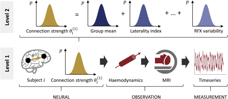
Fig. 1
Full legend
The two-level Parameter Empirical Bayes (PEB) model used in our analysis. At the first level (bottom of the figure), a forward model (DCM) describes how neural activity causes the fMRI timeseries of each subject i=1…N. The parameters from the neural part of the model are taken to the group level (upper part of the figure), where they are modelled as a linear combination of a group mean, a group difference due to laterality index, covariates of no interest (not shown) and random effects (RFX) variability. Image credits: “Brain image” by parkjisun and “CT Scan” by Vectors Market from the Noun Project.
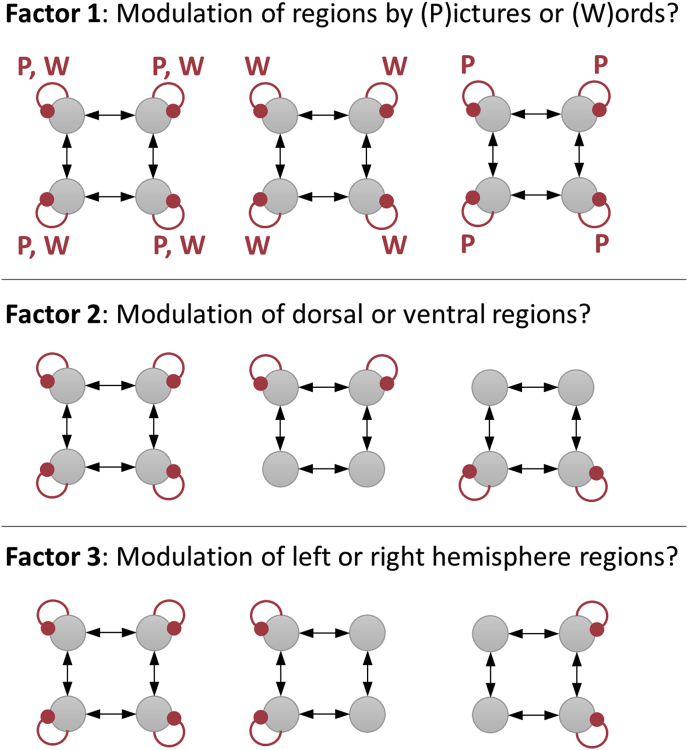
Fig. 2
Full legend
Model space. Each picture is a network of four frontal brain regions. The grey circles in the top row of each picture are left dorsal (ldF) and right dorsal (rdF) frontal cortex, and the circles in the bottom row of each picture are left ventral (lvF) and right ventral (rvF) frontal cortex. The red curved lines indicate inhibitory self-connections that were allowed to be modulated by the task. Candidate PEB models varied according to the three factors shown. Additionally, a ‘null’ model (not shown) was specified with no modulation to serve as a baseline. This gave rise to 3×3×3+1=28 models.
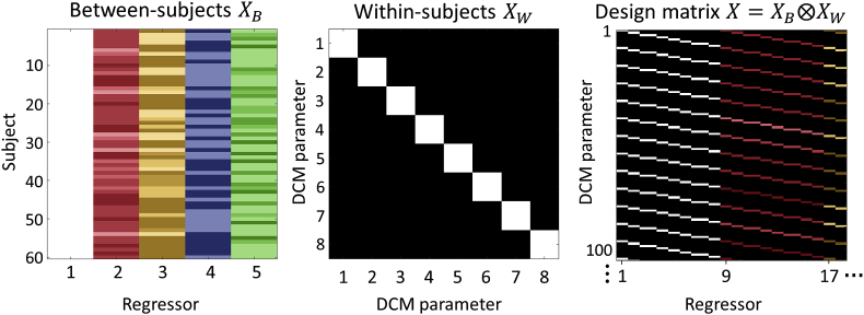
Fig. 3
Full legend
The group-level design matrixX. Left: the between-subjects design matrix, with regressors (covariates) modelling the group mean, laterality index, handedness, gender and age. Middle: the within-subjects design matrix, where the diagonal encodes which DCM parameters receive group-level effects. This was set to the identity matrix to include all between-subject effects on all DCM parameters. Right: The resulting design matrix, computed according to Equation (5). Each row corresponds to one DCM parameter from one subject and each column corresponds to one group-level effect (e.g. gender) on one DCM parameter. For display purposes only, the regressors were z-scored and thresholded to produce colours in a consistent range.
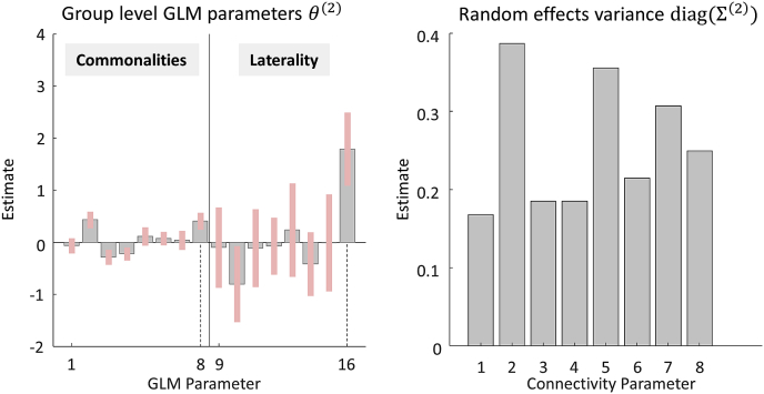
Fig. 4
Full legend
Parameters of the group-level Bayesian General Linear Model (GLM). Left: the posterior parameter estimates, corresponding to the first 16 regressors in design matrix X. These represent the commonalities (average) across subjects (GLM parameters 1–8) and the difference in connectivity due to Laterality Index (LI, GLM parameters 9–16). The units are the same as the parameters in the underlying DCMs; i.e., unitless log scaling parameters that scale the default self-connection strength of −0.5Hz. Dotted lines indicate parameters relating to the modulation of region rdF by words, discussed in the text. Right: the estimated between-subject variance of each connectivity parameter, after accounting for known effects. Parameters have the same order in both plots: 1 = Modulation of lvF by pictures, 2 = ldF by pictures 3 = rvF by pictures, 4 = rdF by pictures, 5 = lvF by words, 6 = ldF by words, 7 = rvF by words, 8 = rdF by words.
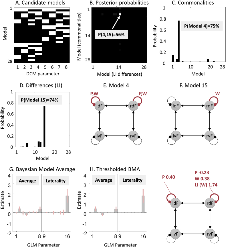
Fig. 5
Full legend
Comparison of PEB models in a pre-defined model space. A. Connectivity parameters switched on (white) and off (black) in each model. See the legend of Fig. 4 for the identity of each parameter. B. Joint probability of all candidate models. The axes list the 28 candidate models (combinations of connections) in terms of commonalities across subjects and differences between subjects due to Laterality Index (LI). In other words, the PEB model in row i column j had parameters relating to commonalities across subjects set according to model i, and parameters relating to LI set according to model j. The best model was number 4 for the commonalities and 15 for laterality differences, with 56% posterior probability. C. The same result shown in part B, summed over the columns and re-normalized, to give the posterior probability for the commonalities across subjects. D. The same result shown in panel B, summed over the rows and re-normalized, to give the posterior probability for the models of laterality index (LI). E-F. Schematic diagrams of models 4 and 15. Curved lines are self-connections modulated by words and/or pictures. G. Bayesian Model Average (BMA) of the parameters over all models. H. The BMA thresholded at posterior probability >95% for clarity. The schematic illustrates the parameters which survived thresholding. P=Pictures, W=Words, LI = Laterality Index.
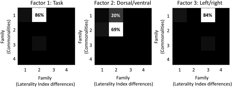
Fig. 6
Full legend
Family-wise analyses for each of three experimental factors. Each plot is a separate analysis with the same 784 PEB models grouped into different families. For each plot, element Pm,n represents the pooled probability for models in which the commonalities parameters were set according to family m and the Laterality Index (LI) parameters were set according to family n. For example, for Factor 1, element P1,2 is the pooled probability for all models with commonalities parameters set according to family 1 and Laterality Index parameters set according to family 2. The families numbered 1–4 for each analysis were as follows. Factor 1 (task): 1 = pictures and words, 2 = words, 3 = pictures, 4 = none. Factor 2 (dorsal/ventral): 1 = dorsal and ventral, 2 = dorsal, 3 = ventral, 4 = none. Factor 3 (left/right): 1 = left and right, 2 = left, 3 = right, 4 = none. See Fig. 2 for an illustration of each factor.
Show all 9 figures
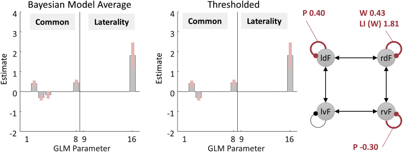
Fig. 7
Full legend
BMA performed on the final 256 models of an automatic parameter search. Left: Posterior parameter estimates based on the BMA. Only parameters relating to commonalities and Laterality Index are shown. Middle: Thresholded BMA, where parameters with probability greater than 95% of being present vs. absent were retained. Each parameter's individual probability was assessed by comparing the evidence for all models (from the final iteration of a greedy search) which had the parameter switched on, versus all models which had the parameter switched off. Right: The schematic shows effects of Pictures (P), Words (W) and Laterality Index (LI).
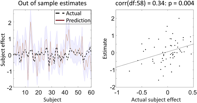
Fig. 8
Full legend
Leave-one-out cross validation. Left: the out-of-samples estimate of (mean-centred) Laterality Index for each subject (red line) with 90% confidence interval (shaded area). The black dashed line is the actual group effect. Right: The actual subject effect plotted against the expected value of the estimated subject effect.
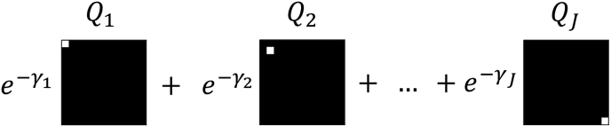
Fig. 9
Full legend
The form of the precision components. Each component Qj has a single non-zero entry at element (j,j), which is set to 16. These are scaled by the corresponding log scaling parameters γj. See Equation (10) for further details.
References30
- 5.
- 8.
- 14.
- 15.
- 17.
- 23.
- 25.
23 more references, whose wording the paper’s licence keeps private.
Cited by papers we hold1
Reads
Read by people on this page
None yet.
Checked or read by AI through naulon
None yet.
A person counts once a day per paper. We keep no cookie and no address: a reader is a hash that changes every day. Any month under five reads shows no number.
Are you an author?
Is this your paper?
Claim it to add your note and be paid when agents cite it. Free.